abstract

University education has become an integral and basic part of most people preparing forworking life. However, placement of students into the appropriate university, college, or disciplineis of paramount importance for university education to perform its role. In this study, variousexplainable machine learning approaches (Decision Tree [DT], Extra tree classifiers [ETC], Randomforest [RF] classifiers, Gradient boosting classifiers [GBC], and Support Vector Machine [SVM])were tested to predict students’ right undergraduate major (field of specialization) before admissionat the undergraduate level based on the current job markets and experience.

Step 1 Pre-processing

we applied different preprocessing techniques by using the Python module, such as removing missing records, deleting irrelevant student records, normalzation, outlier detection, and hot encoding. To increase the proposed system performance,we also created new features by creating different categories at different education levels(ssc_p_catg, hsc_p_catg, mba_p_catg, degree_p_catg and etest_p_catg). To remove the missing records, we used different missing record techniques. Sometimes, ML techniques do not process the categorical technique; therefore, we applied the hot encoding technique.

1-Import libaray

import numpy as np 
import pandas as pd 
import seaborn as sns 
import matplotlib.pyplot as plt
from prettytable import PrettyTable
from sklearn.metrics import roc_curve, auc
from mlxtend.plotting import plot_confusion_matrix 
from sklearn.model_selection import train_test_split
from sklearn.metrics import classification_report, confusion_matrix
from sklearn.tree import DecisionTreeClassifier
from sklearn.ensemble import RandomForestClassifier
from sklearn.svm import LinearSVC
from sklearn.linear_model import LogisticRegression
from sklearn.neighbors import KNeighborsClassifier
import warnings
warnings.filterwarnings("ignore")

2- Data Loading

from google.colab import drive
drive.mount('/content/drive')
import pandas as pd
import numpy as np
data = pd.read_csv("/content/drive/MyDrive/Datasets/Student field Recommendation /Placement_Data_Full_Class.csv")
data.size
data.head()

3-Preprocessing

3.1 Creating Category of Mark Secured in Different Educational Phase
Here we will create 3 category:

• 85% +
• 60% — 85%
• < 60%

def checkCateg(perct):
    if(perct >= 85):
        return '85% +'
    elif(perct < 85 and perct >= 60):
        return '60% - 85%'
    else:
        return '< 60%'
data['ssc_p_catg'] = data['ssc_p'].apply(checkCateg)
data['hsc_p_catg'] = data['hsc_p'].apply(checkCateg)
data['mba_p_catg'] = data['mba_p'].apply(checkCateg)
data['degree_p_catg'] = data['degree_p'].apply(checkCateg)
data['etest_p_catg'] = data['etest_p'].apply(checkCateg)
data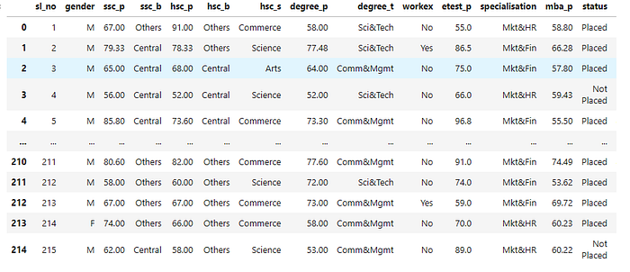

3.2 -Check Missing Value

total = data.isnull().sum().sort_values(ascending=False)
percent = (data.isnull().sum()/data.isnull().count()).sort_values(ascending=False)
missing = pd.concat([total, percent], axis=1, keys=['Total', 'Percent'])
missing.head(4)
output
 Total Percent
salary 67 0.311628
etest_p_catg 0 0.000000
degree_t 0 0.000000
gender 0 0.000000
data = data.dropna(axis = 0, how ='any')
np.sum(data.isnull().any(axis=1))

3.3-Hot Encoding

data.select_dtypes(include=['object']).columns
Index([], dtype='object')
data['gender'] = data['gender'].fillna(data['gender'].mode()[0])
data['ssc_b'] = data['ssc_b'].fillna(data['ssc_b'].mode()[0])
data['hsc_b'] = data['hsc_b'].fillna(data['hsc_b'].mode()[0])
data['hsc_s'] = data['hsc_s'].fillna(data['hsc_s'].mode()[0])
data['degree_t'] = data['degree_t'].fillna(data['degree_t'].mode()[0])
data['workex'] = data['workex'].fillna(data['workex'].mode()[0])
data['specialisation'] = data['specialisation'].fillna(data['specialisation'].mode()[0])
data['status'] = data['status'].fillna(data['status'].mode()[0])
data['ssc_p_catg'] = data['ssc_p_catg'].fillna(data['ssc_p_catg'].mode()[0])
data['hsc_p_catg'] = data['hsc_p_catg'].fillna(data['hsc_p_catg'].mode()[0])
data['mba_p_catg'] = data['mba_p_catg'].fillna(data['mba_p_catg'].mode()[0])
data['degree_p_catg'] = data['degree_p_catg'].fillna(data['degree_p_catg'].mode()[0])
data['etest_p_catg'] = data['etest_p_catg'].fillna(data['etest_p_catg'].mode()[0])
from sklearn.preprocessing import LabelEncoder
lencoders = {}
for col in data.select_dtypes(include=['object']).columns:
    lencoders[col] = LabelEncoder()
    data[col] = lencoders[col].fit_transform(data[col])
data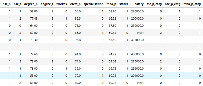

3.4-Feature Scaling

# Standardizing data
from sklearn import preprocessing
r_scaler = preprocessing.MinMaxScaler()
r_scaler.fit(data)
data = pd.DataFrame(r_scaler.transform(data), index=data.index, columns=data.columns)

3.5-Data spliting

X=data.drop('specialisation',axis=1)
y=data[['specialisation']]
X_train, X_test, y_train, y_test = train_test_split(X, y, test_size=0.30, random_state=100)

Feature Selection

!pip install boruta

from boruta import BorutaPy
from sklearn.ensemble import RandomForestRegressor
import numpy as np
forest = RandomForestRegressor(n_jobs=-1,max_depth=5)

boruta= BorutaPy(estimator= forest, n_estimators='auto',max_iter=100)
boruta.fit(np.array(X),np.array(y) )
green_area= X.columns[boruta.support_].to_list()
blue_area= X.columns[boruta.support_weak_].to_list()

print('Feature in green ara:',green_area)
print('Feature in blue ara:',blue_area)

#Calculating Features Importance
def Calculating_Entropy(Labels):
    Calculating_Entropy=0
    labelCounts = Counter(Labels)
    for label in labelCounts:
        probability_of_label = labelCounts[label] / len(Labels)
        Calculating_Entropy -= probability_of_label * math.log2(probability_of_label)
    return Calculating_Entropy

def Calculating_Information_Gain(str_labels, split_labels):
    Calculating_Information_Gain = Calculating_Entropy(str_labels)
    for branch_subset in split_labels:
        Calculating_Information_Gain -= len(branch_subset) * Calculating_Entropy(branch_subset) / len(str_labels)
    return Calculating_Information_Gain

def data_split_for_label(dataset, column):
    data_split = []
    col_vals = data[column].unique() 
    for col_val in col_vals:
        data_split.append(dataset[dataset[column] == col_val])
    return(data_split)
from collections import Counter
import math
IN_gain=[]
Feature_Names=[]
def Results_of_Information_Gain(dataset):
    b_gain = 0
    b_feature = 0
    features = list(data.columns)
    features.remove('specialisation')
    for feature in features:
        data_split = data_split_for_label(data, feature)
        labels_split = [dataframe['specialisation'] for dataframe in data_split]
        gain = Calculating_Information_Gain(dataset['specialisation'], labels_split)
        print(' \n')
        print('-------------------------------------------------------------------------------------------------')
        print('-------------------------------------------------------------------------------------------------')
        print(feature)
        print(gain)
        IN_gain.append(gain)
        Feature_Names.append(feature)
        print('-------------------------------------------------------------------------------------------------')
        print('-------------------------------------------------------------------------------------------------')
        if gain > b_gain:
            b_gain, b_feature = gain, feature
    return b_feature, b_gain

new_data = data_split_for_label(data, Results_of_Information_Gain(data)[0])
IG=pd.DataFrame()
IG['Features Importance']=IN_gain
IG['Features Importance']=round(IG['Features Importance'],2)
IG['Feature']=Feature_Names
IG=IG.sort_values(by=['Features Importance'], ascending=False)
Features_Group = IG[IG['Features Importance'] > 0.1]
print('Length of group features', len(Features_Group))
     
Length of group features 6

print('Selected Features in group:\n\n', Features_Group['Feature'])
Group_Features_Data=data[list(Features_Group['Feature'])]

Group_Features_Data

ExtraTreesRegressor

from sklearn.ensemble import ExtraTreesRegressor
from sklearn.model_selection import train_test_split
from sklearn.metrics import accuracy_score as acc

reg= ExtraTreesRegressor()

     

reg.fit(X_train,y_train)

     
ExtraTreesRegressor(bootstrap=False, ccp_alpha=0.0, criterion='mse',
                    max_depth=None, max_features='auto', max_leaf_nodes=None,
                    max_samples=None, min_impurity_decrease=0.0,
                    min_impurity_split=None, min_samples_leaf=1,
                    min_samples_split=2, min_weight_fraction_leaf=0.0,
                    n_estimators=100, n_jobs=None, oob_score=False,
                    random_state=None, verbose=0, warm_start=False)

reg.feature_importances_
feat_importances = pd.Series(reg.feature_importances_, index=X_train.columns)
feat_importances.nlargest(5).plot(kind='barh')
plt.show()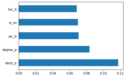

Data Exploring

data.hist(figsize=(50,50),bins = 20, color="#107009AA")
plt.title("Features Distribution")
plt.show()

import numpy as np # linear algebra
import pandas as pd # data processing, CSV file I/O (e.g. pd.read_csv)
import matplotlib.pyplot as plt # Data visualization
import seaborn as sb 
from itertools import product
%matplotlib inline

# Value of count of different Specialization
data['hsc_s'].value_counts()
# Visualization of higher secondary specialization
cls_name = ['Commerce', 'Science', 'Arts']
fig, ax = plt.subplots(figsize = (14.7, 8.27))
wedges, text, autotext = ax.pie(data['hsc_s'].value_counts(), labels = cls_name, autopct = '%1.2f%%')
ax.legend(wedges, cls_name, loc = "center left", bbox_to_anchor =(1, 0, 0.5, 1))
ax.set_title("Proportion of Different Specialization in Higher Secondary");

# Visualization of higher secondary specialization
cls_name = ['Commerce', 'Science', 'Arts']
fig, ax = plt.subplots(figsize = (14.7, 8.27))
wedges, text, autotext = ax.pie(data['hsc_s'].value_counts(), labels = cls_name, autopct = '%1.2f%%')
ax.legend(wedges, cls_name, loc = "center left", bbox_to_anchor =(1, 0, 0.5, 1))
ax.set_title("Proportion of Different Specialization in Higher Secondary");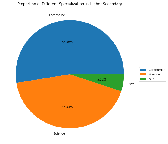

# Visualization of Degree Specialization
fig, ax = plt.subplots(figsize = (14.7, 8.27))
wedges, text, autotext = ax.pie(data['degree_t'].value_counts(),
                                labels = data['degree_t'].value_counts().index, 
                                autopct = '%1.2f%%')
ax.legend(wedges, data['degree_t'].value_counts().index,
          loc = "center left", bbox_to_anchor =(1, 0, 0.5, 1))
ax.set_title("Proportion of Different Specialization in Degree");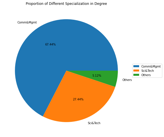

# Visualization of Postgrad Specialization
fig, ax = plt.subplots(figsize = (14.7, 8.27))
wedges, text, autotext = ax.pie(data['specialisation'].value_counts(),
                                labels = data['specialisation'].value_counts().index, 
                                autopct = '%1.2f%%')
ax.legend(wedges, data['specialisation'].value_counts().index,
          loc = "center left", bbox_to_anchor =(1, 0, 0.5, 1))
ax.set_title("Proportion of Different Specialization in Post Graduation")
     
Text(0.5, 1.0, 'Proportion of Different Specialization in Post Graduation')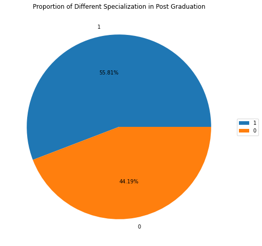

Please Follow and 👏 Clap for the story courses teach to see latest updates on this story

If you want to learn more about these topics: Python, Machine Learning Data Science, Statistic For Machine learning, Linear Algebra for Machine learning Computer Vision and Research
Then Login and Enroll in Coursesteach to get fantastic content in the data field.
📚GitHub Repository
📝Notebook